Defining Boundary Conditions
The software defines two boundary conditions (BCs) on every model. These are applied to reference points (RPs) which are tied to suitable geometry using multi-point constraint equations. They are as follows:
An Encastre (fixed) boundary condition is defined on the ‘RP-1-set’ reference point. This means that all points tied to this RP are fixed in all translational and rotational directions. This BC is applied starting from the Initial step.
A second boundary condition is applied in the first (and only) step on the ‘RP-1-set’ reference point. Currently, the following loadings are available:
Uniaxial Monotonic Displacement BC: Only one value is required.
Uniaxial Monotonic Concentrated Force: Only one value is required.
It should be noted that the of the loading influences the ribbons created for the structure (see Assembling the Unit Cells). The boundary condition is applied based on Structure Type defined when creating the structure. See Different Structure Modes for a list of structure types and the boundary conditions applied to them.
When running a batch analysis, these parameters are used for all models. If a model needs different boundary conditions, it should be run as a separate analysis.
Defining Boundary Conditions using the GUI
The Loading Parameters frame of the analysis tab can be seen in Fig. 10.
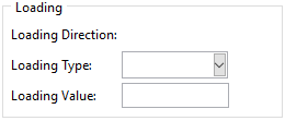
Fig. 10 The loading parameters frame.
Defining Boundary Conditions using the API
Job parameters are defined by defining a LoadingParams object. A list of all attributes and their significance can be found in classes.auxetic_structure_params.LoadingParams. An example is shown below:
# Define the loading_params object
# for a displacement in the x direction.
loading_params = LoadingParams(
    type      = 'disp',
    direction = 'x'   ,
    data      = 20.0
)